Critical community sizes in epidemics

I was reminded the other day of an interesting concept I read about sometime ago, called the critical community size of an epidemic. The idea, first introduced by Bartlett [1], is that a community must be of a certain size in order for an epidemic to persist indefinitely (that is, the size required for an epidemic to become endemic). Bartlett first discussed this idea in the context of measles, in which he theorized the critical community size of measles is between 250,000-300,000 people. Any measles epidemic in a community with a population less than this would eventually "fadeout," or disappear. This is because the number of susceptibles in the population decline until eventually reaching an amount insufficient to allow for continued spread of the pathogen!

Although some of the conclusions presented in [1] have been debated since its publication (see e.g. the discussion in [2] for details), the fundamental takeaway remains interesting. Many scientists (and news outlets, it would seem) lean heavily on the basic reproduction number of a disease in order to assess its capability to spread in a population. The truth of the matter is, however, that there are many numeric quantities that allow scientists to characterize a disease. Although not as popular, the critical community size still helps us understand the capability of a disease to remain in a population - a piece of information regretfully ignored if we were to only look at the basic reproduction number. I'm not downplayig the utility of this constant, I'm merely stating that there is much more to an epidemic than a single number!

To help intuit the idea of a crtical community size a little more clearly, I wrote a program for a discrete-time SIRS model that takes place on a square grid. Each individual in the grid makes contact with their four cardinal neighbors - above, below, left, and right. The individuals contact all four of their neighbors only once per time step. Upon contact, infectious individuals will transmit the disease with probability $\beta$. If disease transmission is successful, infectious people will recover with probability $\gamma$. Recovered individuals eventually lose immunity with probability $\delta$ during each time step. An example simulation of the grid model is given in Figure 1. Note how even if the assumption of temporary immunity is relaxed, the susceptible population can still be replenished by processes of e.g. birth or immigration. Elaborating on his ideas, Bartlett used a discrete-time SI model in his original paper, assuming that the susceptible population was replenished at a constant rate.

Since the model is discrete, events are distributed geometrically. That is, taking recovery as an example, if individuals recover with probability $\gamma$ per time step, then the probability that they recover $x$ days following infection is $(1-\gamma)^{x-1}\gamma^x$. The average infectious period is then $1/\gamma$ and, similarly, the average time that an individual possesses immunity is $1/\delta$. These results are nice, as they're similar to what we'd expect under the assumption of constant rates in continuous-time ODE models. However, this is the extent of the "niceness," as discrete-time models tend to be a lot more difficult to analyze! Some of this complexity is explained in a previous post.

Getting back to the model, we can approximate the critical community size of our system by looking at when fadeout is the predominant outcome of the epidemic. Although there is no standard from which to go by, we can set the threshold at $50\%$ for the sake of demonstration. It should be noted that even successful epidemics can die off just due to the stochastic nature of the simulation. That being said, it helps to have a large numbers of simulated epidemics to go off of - a small sample size isn't useful if the goal is prediction. I settled at only 100 simulations, although I admit this is rather small - I usually go with at least 200 simulations, but I had to use my laptop for a project I had due the week I made this post. Finally, since it's near impossible to determine permanence in a discrete-time simulation, I set the cutoff point at two years. Therefore, any epidemic that made it to the two year mark is assumed permanent. The population in the simulation is varied by changing the side lengths of the grid, so that data points are all square numbers. The results for each population are plotted in Figure 2.

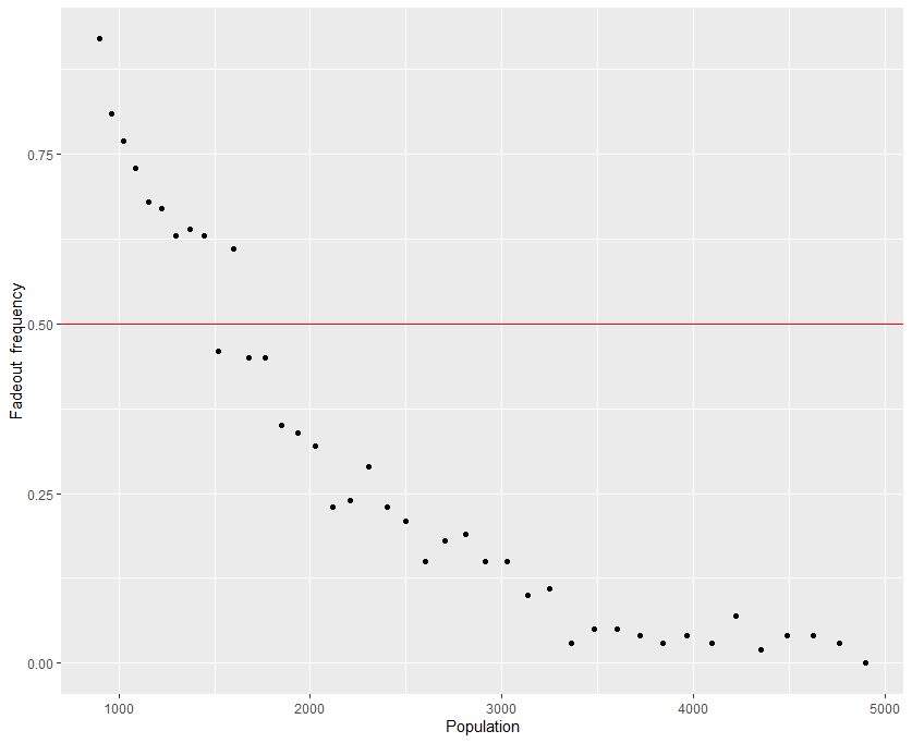
Based on the results of the stochastic simulations, the critical community size of the hypothetical disease is around $39^2 - 42^2$, or a population of anywhere from 1521 to 1764. Below this population the epidemic will fadeout within two years, while above this population it will persist a majority of the time. As the population becomes larger, fadeouts become more infrequent over the course of the two years.

Indeed, what is meant by "community" is quite debatable, as a community in western Europe may not look or behave like a community in southeast Asia. Even more, communities worldwide have changed quite dramatically since the year that Bartlett originally formulated the concept! Such a metric is still useful, however, as it tells us how transmissible a disease is (measles has a much higher critical community size than, say, influenza, as the former spreads much more rapidly and therefore needs a large number of susceptible humans to maintain permanence), and the endemic potential a pathogen has in a general human community. The idea of a critical community size does have its limitations, however. Most importantly, it only makes sense for non-zoonotic diseases. This is because the assumption of a critical community size is that the success of an epidemic (speaking strictly in terms of persistence) depends on the size of the human population, and that transmission in that population only depends on human agents. A zoonotic disease, however, does not require a human host to thrive, and so applying this concept to the study of a zoonosis would be nonsensical. The pathogen must also be transmitted via a human to human pathway. Malaria is a good illustration of this, as it cannot be transmitted from human to human, and so the depletion of susceptibles does not rely solely on the density of humans in a community.

References

[1] Bartlett, M.S. The Critical Community Size for Measles in the United States. Journal of the Royal Statistical Society: Series A (General). 1960; 123(1).

[2] Keeling, M.J. & B.T. Grenfell. Disease extinction and community size: modeling the persistence of measles. Science. 1997; 275(5296).