Batesian butterflies

Take a look at the butterflies in Figure 1. Upon a quick glance, one may be tempted to classify them as the same species. However, this couldn't be farther from the truth! They are actually two different species of butterfly that can be found together in southern regions of Asia. But why do they look so similar? Is this pure chance, or something more?

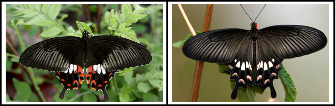
First it helps to know why an organism bothers with these vibrant colorings in the first place. Although this isn't shown in Figure 1, the body of the common rose is a vibrant red. Animals use eccentric coloring as a warning sign to predators (a phenomeon referred to as aposematism). Some familiar examples might be the bright coloration of poison dart fogs, the distinct white-black pattern in the fur of skunks, or the hissing sound that snakes make when threatened (a form of acoustic aposematism). If you've ever had the misfortune of experiencing any of these examples, then you can probably testify as to their effectiveness!

Some of these mechanisms are so effective, in fact, that some organisms have evolved to mimic them, without necessarily adapting the protective features behind the warning signs. Enter the common Mormon, shown in the left image of Figure 1. This butterfly species doesn't produce a poison like the common rose butterfly, so it is perfectly edible, but because of its coloring predators will avoid it nonetheless. This is an example of Batesian mimicry, or when a palatable or undefended species (the ‘mimic’) resembles an unpalatable or otherwise defended species (the ‘model’), and thereby gains protection from predators [1]. To keep things general, I'll be using this nomenclature from this point forward. Admittedly, it can be confusing talking about a mathematical model of interactions between a ‘model’ and a ‘mimic’, but I'll make it clear as to which model I'm referring to. I should also mention here that the predator species fooled by the mimic is referred to as the ‘dupe’.

This sounds like an excellent way to avoid predators without going through the expense of evolving your own form of protective mechanisms, but there is a glaring drawback: the coloring is only protective insofar that predators actually associate it with a defense. Specifically, if you were to take common Mormon butterflies and place them into an ecosystem where the common rose is entirely absent, they would be devoured. In this way, the advantage is said to be frequency-dependent. We can expect a similar outcome if there are too many common Mormon butterflies, or too few common roses. Just how many model organisms are required to ensure persistence of the mimic, and what relationships can we see between both populations? Sounds like the perfect question to answer using mathematics...

Prior to any equations, I always find it helpful to look at how the system behaves from an agent-based perspective. Not only because NetLogo is an excellent and easy language to use, but behaviors gleaned from agent-based models can help inform the mathematics moving forward.

Originally, I thought about keeping the predator species constant, as the idea of a frog species feeding only on butterflies seemed silly. Eventually I realized that the predator population should be modeled as well, as consumption of the model species can kill the predator (especially if the model species is poisonous).

The species in our system are then the model, the mimic, and the predator. Because the mimic is so good at playing copycat, the predator is unable to discern between either prey species. That being the case, the model and mimic are preyed upon by the predator at rates proportional to their respective populations assuming random mixing -- absolutely no preference is allowed. Finally, we assume the model and mimic compete for different resources. This isn't totally outlandish, as some model species in nature will have a unique diet as required by their defense mechanism (the common rose being a good example of this -- the plants it consumes as a larva make it poisonous to predators). A system of ordinary differential equations taking all this into account will look something like as follows:

The state variables in our system are the model species, $x$, the mimic species, $y$, and the predator, $p$. We take the growth rate of the model and mimic species to be $\lambda_1$, $\lambda_2$, and the carrying capacities of each to be $K_1$, $K_2$, respectively. The predator population, $p$, preys upon either species at a rate $\alpha(x,y)$. The consumed prey species are converted to new predators according to the constant $c$. Note how only consumption of the mimic species contributes to the growth of the predator population, as consumption of the model species (the one that's actually dangerous!) results in the death of the predator. When the model species is consumed, biomass is removed rather than added. Besides this, the predator dies at a constant rate of $\mu$.

The predation rate $\alpha(x,y)$ is a function of both prey species as it depends on their frequencies in the environment. The predation rate will decrease as the model species increases, as the predator will be conditioned to avoid eating the prey. In the reverse direction, the rate will increase with the frequency of the mimic species because no negative conditioning occurs. For simplicity, we take $$0 = \alpha_{min} = \alpha(K_1,0) \le \alpha(0,K_2) = \alpha_{max} = \delta.\nonumber$$ In general, the following conditions should hold:

What are some possible functions of $\alpha(x,y)$ that satisfy these restrictions? A simple assumption is that the predation rate increases linearly with the mimic species, and decreases linearly as the model species becomes more abundant. If we agree that the predation rate is zero in the absence of any prey, then the points $(0,0,0)$, $(K_1,0,\alpha_{min})$, and $(0,K_2,\alpha_{max})$ uniquely define a plane with equation $$z = \alpha(x,y) = \alpha_{min}\frac{x}{K_1} + \alpha_{max}\frac{y}{K_2}.\nonumber$$ Using this predation rate, with $\alpha_{min} = 0$ and $\alpha_{max} = \delta$, and \eqref{LV} becomes

Now that we've motivated a mathematical model from the natural phenomena we're interested in studying, what can this tell us? The first step in the analysis of any dynamical system is the identification of equilibria. The system in \eqref{linear} produces the single-species equilibria

as well as the two-species equilibria

and a coexistence equilibrium too long to show here. It is important to mention that since we took $\alpha_{min} = 0$, there does not exist a stable equilibrium where the model and predator are the only species present. There are other equilibria that I have not listed above because these possess negative species counts, which we’re not too interested in from a biological standpoint. The coexistence equilibrium is the most interesting, but the single- and two-species equilibria help us understand the response of the system to changes in parameter values. For example, one may anticipate that the presence of too many mimic species (controlled by changing their carrying capacity, $K_2$) could negate the advantage had my mimicking the model species. This could be catastrophic for the mimic species, or equally catastrophic for the model species if they are unable to contend with higher predation rates in response to mimic abundance.

These questions can be answered by checking the stability of each of the equilibria. This is done by checking the signs of the eigenvalues of the Jacobian evaluated at the respective equilibrium point. For the single-species equilbria, this is straightforward as most of the values cancel out. One easily finds that each of the single-species equilibria is always unstable. If we agree that it is impossible for the populations in the system to explode to infinity (as each either directly or indirectly mediates the size of another), then it must be that at least two populations are present in the system at equilibrium.

Unfortunately, the conventional stability approach described above doesn't help too much when we apply it to the two-species or coexistence equilibria, as things become a bit garbled. Nonetheless, we can attack the problem numerically if we confine ourselves to a certain region of the parameter space. The parameters we will look at are the carrying capacity of the mimic species, $K_2$, and the maximum predation rate, $\delta$. To illustrate what I mean by a numerical study, consider the two-species equilibrium favoring survival of the mimic and predator. Although an explicit form of the equilibrium is hard to work with, checking the signs of the eigenvalues of the Jacobian to determine asymptotic stability is a straightforward process for any computer algebra system (Mathematica, in this case). This way we can identify regions in the $(y^*,p^*)$ plane where the critical point is asymptotically stable or unstable (the asterisk notation here denotes equilibrium value). This gets something like the following plot:

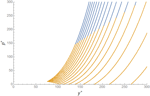
We can see that the asymptotically stable region (where the model species goes extinct) occurs for large predator populations. This tells us that the large predation rate in response to larger abundances of the mimic species is enough to drive the model species to extinction. Well of course! If I were to introduce a few inedible/poisonous butterflies into a population of delicious butterflies, then the frogs could not care less and would carry on eating as they please. However, if the predator population is not as large, then the model species will not tend toward extinction even in the presence of a large population of mimics. The values of $K_2$ and $\delta$ can help us control where on this plane the trajectory will land after we notice that $(y^*, \ p^*) \sim \left( \sqrt{K_2/\delta}, K_2^{3/2}/\sqrt{\delta}\right)$ for sufficiently large $K_2$.

We can repeat this procedure for all of the equilibria we are interested in, and compare their respective stable regions. This will help us better understand their relationship with one another, and clearly identify regions of bistability. Let's increase the resolution of our parameter sweeps to make our plots more surface-like, and juxtapose each stable region on top of the other one in the $(K_2,\ \delta)$ plane, as shown in Figure 4 below.

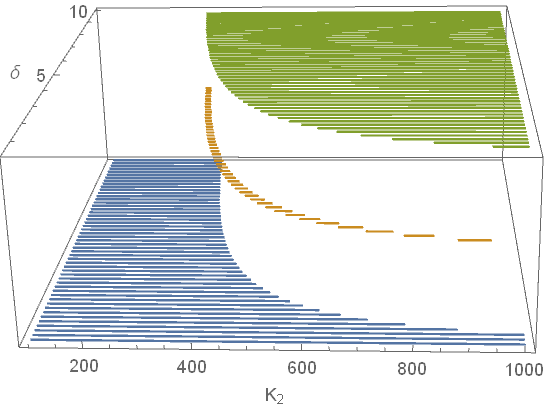
Although it may be hard to tell from Figure 4, there is some overlap between the regions corresponding to areas in the parameter space where the system is bistable. The stable regions for the $yp$ and coexistence equilibria are disjoint, but there are bistable regions for the $yp$ and $xy$ equilbria, and for the $xy$ and coexistence equilbria. In other words, when all species are present at equilibrium, system perturbations can only result in the death of the predator. These perturbations will never result in the extinction of the model species. If only the mimic and predator species are present at equilibrium, then no perturbation to the system will allow for the successful reintroduction of the model without causing the extinction of the predator.

To illustrate what this looks like, we can visualize how the population trajectories respond to progressively greater perturbations (see Figure 5). Initially, the population is at equilibrium with all three populations present (represented by the blue dot). If the predator population is reduced enough, then trajectories will eventually favor extinction of the predator species (represented by the red dot). Population suppression of the predator species can occur as a result of migrational changes due to climate change, habitat disruption, or hunting, to name a few possible reasons.

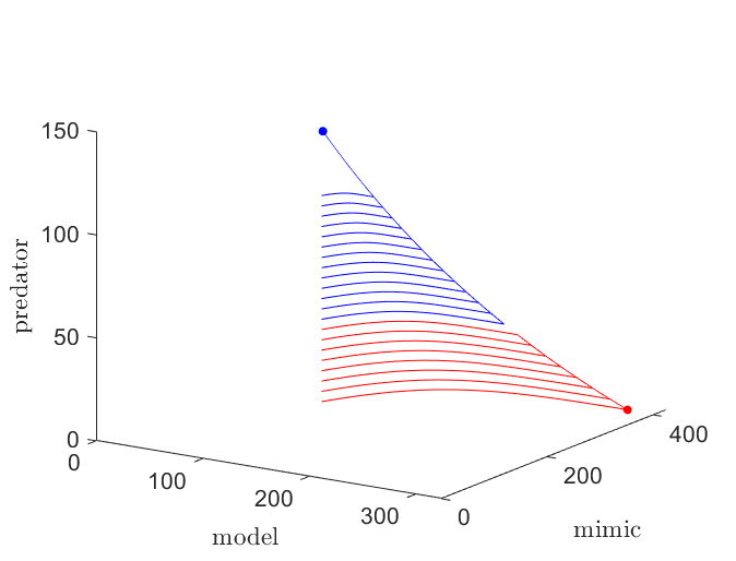
Local extinction of the predator species can be catastrophic to its habitat ecosystem. A predator can serve various essential purposes within their environment, so it is hard quantifying the consequences to be had if extinction were to occur. A role that we considered in \eqref{linear} is the role of regulating prey species populations. If the predator goes extinct then, left unchecked, these populations balloon in size, as seen in Figue 5. Explosive population growth places immense pressure on the local ecosystem, and could spell bad news down the line for organisms the prey species are reliant on for survival.

Looking back at Figure 4, another takeaway is that lower mimic abundance (smaller $K_2$) favors coexistence between the mimic and model species. As we saw above, if there are too many mimics, the model species is unable to recover from the increased predation rates and will go extinct. This has to do with how we set up our model, specifically our assumption that predation increases linearly in the presence of the mimic species. We made this assumption because the system was simpler, but what if we used a different form of $\alpha(x,y)$? If we put ourselves into the position of the predators, and happened to snack on a particularly foul tasting butterfly, chances are we wouldn't be too willing to snack on another! That is to say, the experience of snacking on a foul or poisonous organism is much more memorable than snacking on a tasty one. We can model this by making it so that the predation rate $\alpha(x,y)$ grows slowly for increasing concentrations of the mimic species and decreases at a quicker rate for increasing abundances of the model species.

However, I've quite a bit of other work on the horizon as well as a conference to prepare for, so I'll cut off the exploring here and leave it to another post down the line to pick up where I left off. This whole mini-project grew out of an idea I had a few weeks ago, but now I must resist putting more time into this in order to redirect my energies elsewhere. Hopefully this has piqued your interest in Batesian mimicry, as well as give you an idea about how catastrophes in natural systems can be studied using mathematics!

References

[1] Finkbeiner, S.D, Salazar, P.A., Nogales, S., Rush, C.E., Briscoe, A.D., Hill, R.I., Kronforst, M.R., Willmott, K.R., & S.P. Mullen. Frequency Dependence Shapes the Adaptive Landscape of Imperfect Batesian Mimicry. Proceedings of the Royal Society B. 2018; 285.