The Blobbian Biosphere

In the game agar.io, you navigate a circular blob in an environment populated by nutrients and other players. Consuming either of these increases the mass of your blob. The object of the game is to consume enough to become the largest blob. Although simple, those who have played it can attest to its addictive qualities. How do agents following such a simple ruleset provide for such an entertaining experience? Moreover, how does such stimulating behavior emerge from a system with so few rules? Ever since I first played this game, I've thought about programming my own version. However, the strategic aspect was more appealing than the gameplay. How often should you play passive rather than aggressive? Is foraging for particles of food across the landscape more efficient than hunting other players?

While back in Maine for a few weeks this past summer, I set aside some time to get a program up and running to tackle these questions. I've also been meaning to program a genetic algorithm for one of my projects recently, as my past few attempts at it have been rather underwhelming. This seemed like the perfect opportunity to kill two birds with one stone.

I have received requests to include what programming languages I use in these posts. From now on, I will be including the languages I use for each project in a (blue) box like this. Also starting with this post, I will be posting my code on GitHub. The code for the program in this post can be found here. Programming languages used in this post: NetLogo, R (ggplot2, lattice).

I finished the program pretty quickly. Things slowed down when I started running batch jobs in NetLogo. The extra laptop I have came in handy for these parts. Now to the actual details of the program. Instead of players, the environment of my program is inhabitated by ``blobs.'' Each blob is endowed with a small set of instructions to follow in response to certain stimuli. How each blob behaves is determined completely by its genome. The genome determines how each blob hunts, forages, chases prey, and breeds. Each task that the blob performs costs energy. Blobs obtain energy by consuming other blobs or nutrients that can be found scattered across the landscape. Too little energy and the blobs die, while an excess amount of energy means the blobs can reproduce if they find a suitable mate.

For those interested in the specifics of the ruleset each blob follows, they can check out the algorithm details in the next section. For now, the only rules that matter are the following:

• the size of a blob determines it's speed and max energy,
• smaller blobs move at greater speeds but have small energy pools, while larger blobs move slower but possess large energy pools,
• certain blob features, such as size, incur energy costs corresponding to their maintenance.

As a quick side note, not really a rule but a convenience: the color of a blob corresponds to its size, i.e. purple is the smallest, followed by blue, green, orange, and red is the largest. That’s all you need to know for now!

At the beginning of a simulation, the environment is initialized with blobs of random genomes (and thus random sizes). For a while, the landscape looks like a Jackson Pollock painting. To encourage convergence to a suitable set of blobbian traits, the mutation probability is set high at the beginning (10%) and is slowly reduced to 2% over the course of a few hundred time steps. Through this trick, the population is given an opportunity to explore a wide breadth of parameter space before settling on one that maximizes fitness. This process is similar to the idea behind simulated annealing. Once the mutation probability settles, many of the blobs die because they are unable to thrive. The few that remain are only able to do so because they've found a combination of parameters allowing survival. These blobs will repopulate the landscape. An example of this happening is shown in Figure 1.

If food is scarce, purple blobs thrive as their greater speed allows for more efficient foraging. When nutrients are more plentiful, the blue and green blobs enter into the fray, both capable of more efficient predation with speedy foraging to boot. As the landscape is repopulated, mutations introduce the larger species back into the environment. The orange and red blobs may forage like their cousin species, but they may also evolve fangs to prey on the more abundant smaller species. Their larger energy pools allow for farther travel distance in pursuit of prey. Predators tend to persist as a small proportion of the population.

Now that we have a program working as expected (I hope), how might we use it to explore blobbian evolution? Probably one of the simplest curiosities to explore is how the blobs respond as food scarcity is varied. This can be controlled by the food-prob variable in the NetLogo program, which is just the probability any individual patch grows food. A value of 0.04 means that 4% of patches produce food, a probability of 0.05 means that 5% of patches grow food, etc. What changes would we expect to happen as food becomes more abundant or scarce across the landscape? The most immediate change would probably occur in blob sizes. We can record how each system selects for different blob sizes by looking at the average blob size over the course of the simulation. As the probability of food changes, we'll be able to see any trends that arise. Plots are shown in Figure 2. Each data point is the average of 50 simulations. Only simulations in which the blobs survived more than 1000 time steps were kept. To better illustrate overall trends, local regression plots are also provided.

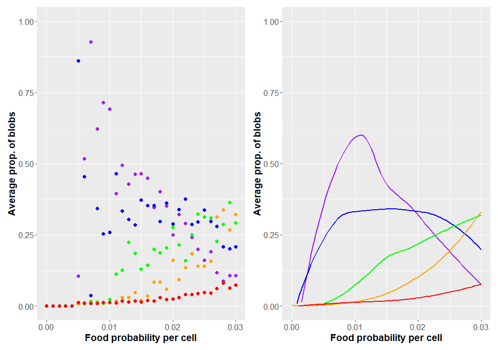
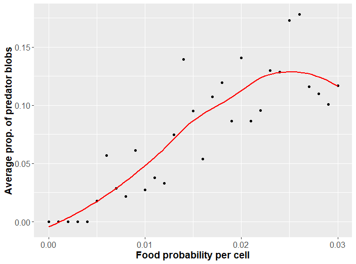
For less bountiful landscapes, faster blobs evolve unrivaled. Greater abundance of food allows larger species to survive. These species can forage themselves or evolve fangs to feed on small prey. Speaking of predation, how might this change with food abundance? Predation evolves when there are sufficiently many other blobs to make such a costly adaptation favorable. A plot of the proportion of predators as food probability changes is given in Figure 3.

There are quite a few scenarios we could explore with this program. Some interesting questions one might ponder are under what conditions larger blobs may evolve? What happens if we increase the mutation rate? At what conditions are the blobs unable to evolve a solution to survive? These latter two questions have to do with an interesting angle of analysis that I pursue more completely next section.

Blobbian evolution within different frameworks

An interesting topic I've seen crop up in my studies recently is the ability of a system to adapt. Adaptation need not be in a biological sense, however. For example, neural networks can learn how to learn. Convolutional neural networks can learn which layers to use where in order to improve performance. The ability of organisms to evolve depends on the parameters of their evolutionary system. Agents in some evolutionary systems are better at evolving than the agents in an alternative system with different parameters. For those interested, Stuart Kauffman's The Origins of Order goes over the latter idea in excellent detail in the context of his own proposed model.

How does this relate to our blobbian world? Well, for all of the analysis up to this point, the parameters governing how blobs evolved have been kept constant. To make things simple, I'll refer to these as hyperparameters. We can view a unique combination of hyperparameters as a point in system space. A change in hyperparameter values corresponds to a different system altogether. For example, what if the mutation rate was changed? What about the carrying capacity? How many alleles change per mutation? How does the capability of the system to evolve change with any of these hyperparameters?

Let's look at this a little more closely. To measure a system's capability to evolve, we can do something similar to how Kauffman answers the same question with his own model in Chapter 5 of the aforementioned text. In particular, we can look at the average blob fitness (determined by energy) over a certain length of time for different systems. The system in which average blobbian fitness is highest is also the system in which the blobs are most capable of adapting to the particular set of environmental conditions. The following hyperparameters are varied: mutation probability and carrying capacity. The average energy as either of these parameters are varied are shown in Figure 4. (From this point on, I will use fitness and energy interchangeably.)

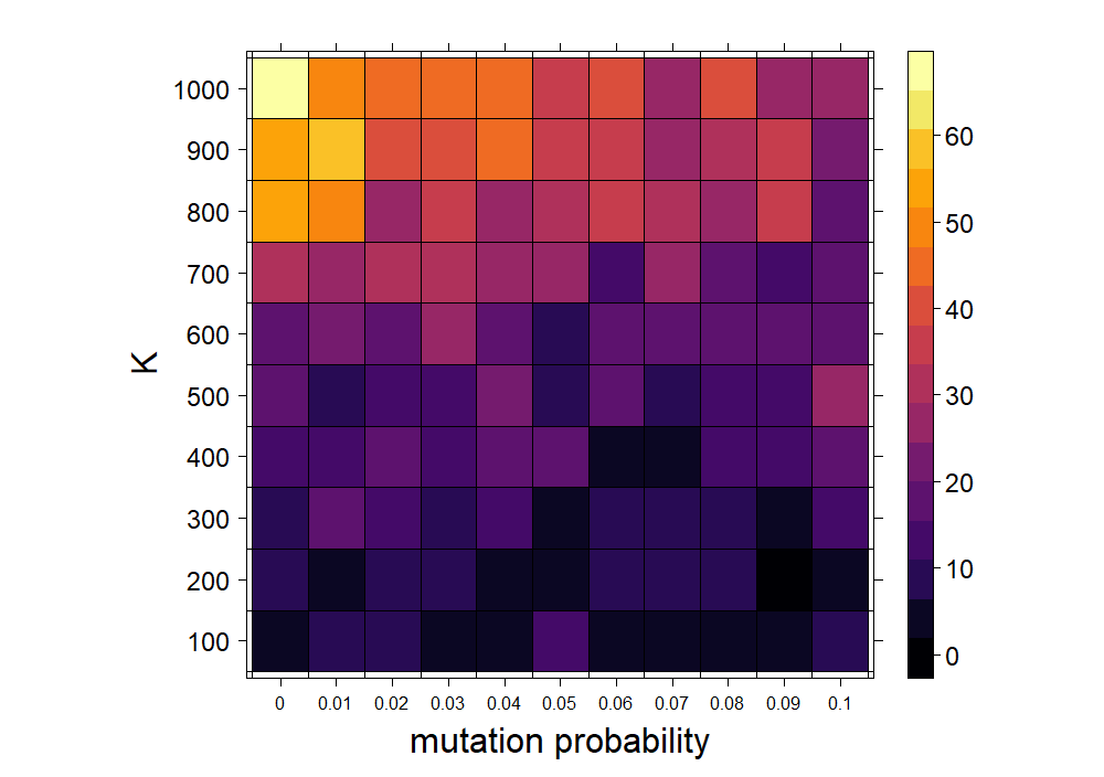
From the plot above, the most dramatic change in energy occurs as the carrying capacity varies. The number of blobs in the system clearly affects their ability to evolve, but more substantially than the mutation rate. This is discussed more fully below. To get a better idea of the contribution of each individual hyperparameter in the previous experiment, we can average across the rows and columns of the matrix of cells in Figure 4. For example, taking the average per row removes variation due to the mutation probability and allows us to look at the contribution of the carrying capacity to the overall mean fitness. This is done in Figure 5.

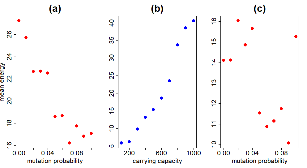
These plots show the correlations much more clearly. Increasing carrying capacity has the opposite effect on the mean energy as increasing mutation probability. Speaking of mutation probability, Figure 5a catches our attention. We would expect an intermediate mutation probability to be optimal. Too high a mutation probability and the system is too volatile; any beneficial combination of genetic traits is short-lived. At the other extreme, too low a mutation probability chokes the system's ability to adequately explore the genotype space, ignoring potentially fitter combinations. Why is this not the case in Figure 5a?

The reason is because we are taking the average over all carrying capacities for each data point. As $K$ becomes sufficiently large, a lower mutation probability is beneficial because of how the system is initialized. At the beginning, each blob is assigned a random genotype, so that the genetic diversity is quite high. Large genetic diversity in the population means less reliance on mutation to introduce or fine-tune beneficial combinations of alleles. This effect disappears if we take the average over a smaller carrying capacity range, as in Figure 5c, where fitness is maximized at an intermediate mutation probability. This quirk is unique to our simulation and not to be expected naturally, both because error-free copying of information is a pipe dream, and organisms are not initialized randomly in nature.

For larger values of $K$ (not shown), fitnesses increase for intermediate mutation probabilities once more. This potentially indicates that blob evolution can rely on random initialization and not mutation for only certain carrying capacities.

The effects of random initialization are more pronounced when one considers how the blobs mate. Mate selection in the blobbian world inherently selects for fitter genotypes. A recurring theme in my work is reconciling with the definition of fitness when used in a particular context. In our case, blob fitness means the ability to acquire a high enough amount of energy in order to breed. Less fit blobs are those unable to reach this energy threshold, and will thus never mate. I guess you could describe it as a sort of sexual selection, where mates will be attracted to fitter genotypes.

Enough about mutation probability -- how does the mean energy change with the carrying capacity? Figure 5b shows the two are heavily correlated. Carrying capacity determines how many offspring are produced during a mating. By default, all blobs produce three offspring. The number of blobs produced during mating is determined by multiplying the number of blobs produced by default and $1-N/K$. Here, $N$ is the number of blobs and $K$ is the carrying capacity. This product is rounded to the nearest integer to determine the number of offspring. Increasing $K$ therefore increases the number of blobs produced during a mating (this leaves our use of the phrase carrying capacity a tad ambiguous -- see final subsection on this).

Blob algorithm at a glance

In this section I'll go over how blobs make decisions. This explanation is copied in the actual NetLogo file of the program, which can be found over on my Github.

First and foremost, blob size determines the most important characteristics of a blob, including speed and maximum energy. Larger blobs move slower than smaller blobs and incur a greater energy cost as well, but have much larger energy pools. Energy is what allows a blob to live and is expended during movement and the daily maintenance of certain blob features, such as fangs and size. If the energy of a blob ever reaches 0, the blob dies. When a blob's energy exceeds it's maxmimum energy, it will search for a mate to breed with. Breeding involves finding another blob that also possesses an energy in excess of it's maximum energy. If a mate is successfully found, the blobs will produce a certain number of offspring. Each offspring trait is inherited from one of the two parent blobs (mutations also occur). Following reproduction, the parent blobs die.

Besides reproduction, blobs have many other tasks they perform. Blobs make decisions by moving down a check list -- a "to-do list" of living, if you will. Before any decision is made, a blob surveys it's neighborhood for a predator blob. Predator blobs are determined by their fang size. A blob is only capable of eating another blob if its fang size is greater than the size of it's prey. For example, a blob with a fang size of 4 can consume blobs of sizes 1 (purple), 2 (blue), and 3 (green). However, larger fangs are more expensive to maintain. If a blob spots a predator blob, it will flee in the opposite direction.

If a predator is not around, the blob will proceed to either hunt or forage based on some genetic probability. If the blob forages, it will survey its surroundings for food. If the blob hunts, it will survey its surroundings for prey. If no food is around, the blob will just amble about. Everything determining movement, including the angles the blobs turn prior to taking any steps, are all determined genetically.

Future changes

There are a few other topics I'd like to write about on this website in the near future. This blob project has been clogging up these plans! Thus, instead of spending more time refining this project and performing more simulations, I resolved on stopping here and including a short section discussing some improvements to be made in the future if I ever return to this project.

A lot of improvements have to do with correcting lazy oversights. For one, the offspring produced following mating are dispersed randomly across the landscape. I thought I would make this change after first spotting it long ago, but I just sort of forgot to do it until recently.

Another thing is the use of two mechanisms of limiting population growth: carrying capacity and finite resources. It would be better to use one and not both simultaneously, as they don't do anything together that they can't accomplish alone. I put in a carrying capacity for the second part as it was easier to envision carrying capacity as the lever we use to control the size of the blob population. Without an explicit carrying capacity, population size is determined by food availability (controlled by the food probability variable). In the future, I should choose only a single mechanism responsible for limiting population growth, as the use of both in the same program is pointlessly complicating.