Barred owls and Béla Bollobás

It is difficult to think that my second year as a graduate student is almost at an end here at NC State. This milestone seems swept up with the turbulence of the present time -- a sentiment I feel is shared by many. Whenever I do enjoy a brief respite, I like to wander back to this website and post a (sometimes) short update, which always just ends up being me talking about something I find interesting.

I have developed a nasty habit of using alliterative post titles. The letter B features prominently, although you must believe me when I say this is completely unintentional. I will leave the more exciting story barred owl story to the end. For now, I want to talk about a wonderful puzzle I recently saw for the first time in years. The puzzle is attributed to the mathematician Béla Bollobás. The rules of the game are summarized in the following blurb:

Consider a $12 \times 12$ grid of squares. Squares can either be infected or susceptible. An infection spreads across this grid: transmission occurs when two infected squares are adjacent to a susceptible square (diagonal neighbors do not count). Squares remain infected for the entire simulation. What is the minimum number of infected squares you need in order to infect the entire grid?

An interesting idea! Interesting to me of course because the question combines three of my most favorite things: disease, math, and programming. Of course, programming the problem is easier than solving it (or is it?). Two example simulations are provided in the figures below (ignore the blue squares in the bottom left—blame R's funcky image function for this one). In the left sim, the grid is initialized with 10 infected squares. A small outbreak proceeds, but fizzles out before spreading terribly far. The sim on the right, however, is a little different: 20 individuals initiate the outbreak which ends up spreading to the entire population.

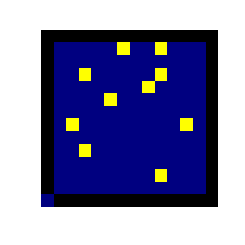
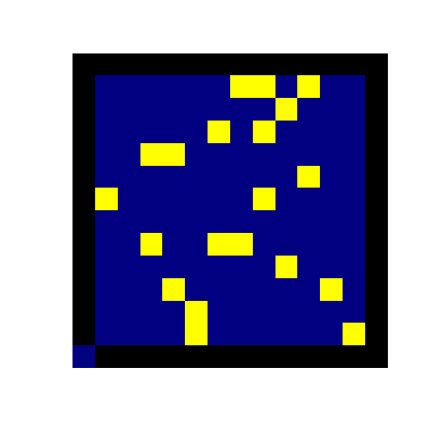
Taking these observations at face value, we have passed a threshold of some kind in the number of initial infected. The sims above give a few hints as to a solution to the problem. Epidemics grow in a rectangular shape, growing to the bounds defined by newly absorbed (infectious) individuals. The growing pattern of these epidemics appear diagonal if one looks close enough; this is especially apparent in the second figure.

Given the rather simple rule set, we can easily explore the behavior of different infection clusters. Some configurations are better than others at producing new infections. If our immediate goal was to produce as many infections in the next generation as possible, how might we accomplish this? Let's limit ourselves to only two infected squares. There are two ways that we can configure two infected squares such that they produce new infections in the subsequent generation. We can place them in a "dotted" pattern, i.e. placing two infected squares so that they lie to either side of a susceptible square. Alternatively, we could also place the infected cells in a diagonal. The latter case results in two new infections in the next generation, while the former secnario will only yield a single new infected square.

Let's do the same for a $3\times 3$ grid. Once again, the scale of the question allows for an easy solution with pen and paper. Perhaps unsurprisingly, the diagonal configuration again comes out on top as one of the configurations most beneficial to the spread of the infection. Three individuals in a diagonal will infect four squares in the next generation. As far as increasing the number of subsequently infected squares is concerned, diagonal configurations perform very well. It can be easily shown that the number of newly infected squares produced from a diagonal of $N$ infected squares is $2(N-1)$.

Is this the most newly infected squares that can be produced in one generation? The answer is yes! The maximum number of newly infected squares that can be produced from $N$ infected squares is $2N$. To see this, note that $N$ infected squares will, at most, have $4N$ sides. If exactly two of these sides yield a new infection, then $2N$ squares will become infected in the next generation. However, this is a little off from the number of new infected squares produced by a diagonal configuration. Where do the extra 2 sides go? Before we go further, we require the following definition and theorem.

Definition: Let the minimum bounding box of a configuration of infected individuals be the smallest rectangle that contains all infected squares.

The minimum bounding box is the set given by $\left[\min\left(\mathbf{X}\right), \max\left(\mathbf{X}\right)\right] \times\left[\min\left(\mathbf{Y}\right), \max\left(\mathbf{Y}\right)\right],$ where $\mathbf{X}$ and $\mathbf{Y}$ are the $x$- and $y$-coordinates of the infected grid cells, respectively. We get the following theorem:

Theorem: An epidemic cannot spread beyond the minimum bounding box of the initial configuration of infected cells.

Proof: (Less a proof and more a heuristic argument:) By our definition of infection, a square can only become infected if it sits between two infected squares, or if it sits in a "corner" formed by two diagonal infected squares. If we assume our square lies on the periphery of such a bounding box, the former case is impossible as no other infected squares lie beyond the bounding box by definition. This leaves the "corner" case as the only possibility of producing new infected squares, which themselves are contained in the minimum bounding box.

So, returning to the above objective of infecting as many squares as possible in a single generation, we now know that an epidemic cannot spread beyond the minimum bounding box of an initial configuration. At mimimum, four sides of initially infected squares will lie on the minimum bounding box and thus not contribute to any new infections. The true maximum number of newly infected squares is then $(4N-4)/2 = 2(N-1)$, which is precisely the number of newly infected produced when we have a diagonal as an initial configuration.

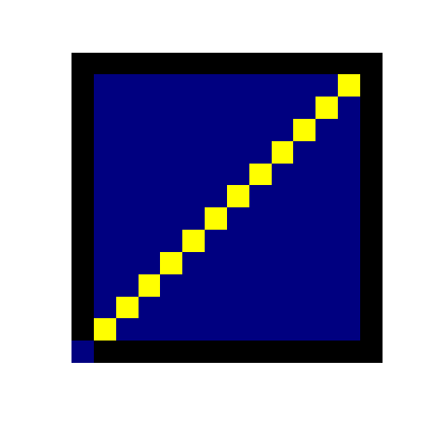
Our argument thus far has demonstrated an initial diagonal configuration performs quite well in the short term, i.e. over a single generation. How does it fare in relation to our initial question relating to a minimal configuration that infects the entire $12\times12$ grid? As it turns out, the diagonal configuration will is actually successful in infecting the entire grid. But does it use the smallest number of squares possible?

Since we want the epidemic to eventually infect the entire population, the minimum bounding box must equal the entire $12\times12$ landscape. This means that our initial configuration must have an infected square in the first and last rows, as well as the first and last columns of the $12\times12$ grid. While four squares easily satisfies these requirements, we could also save two by placing two infected squares in opposite corners of the grid. Now, we want to get the infection from one corner of the grid to the other corner. The easiest way to do this is via the addition of more diagonal units until both opposite corners are connected by a diagonal.

This method uses very few squares (only 12 of the 144), but is it optimal? Yes! In fact, for any $N\times N$ grid, the least number of initially infected squares needed to infect the entire grid is $N$ squares. A succinct proof of this for the $12\times12$ case is as follows: Notice that the perimeter of the overall shape formed by the infected squares cannot increase as more infected squares are added. Because the grid has perimeter $48$, the original configuration must also have a perimeter of $48$. The smallest number of squares satisfying this requirement is $48/4 = 12$ squares.

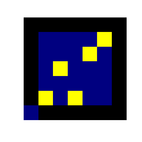
Our diagonal configuration above only contains $12$ squares. It should be made clear that the proof above does not rule out alternative configurations; it just requires that these configurations must use only $12$ squares. A non-diagonal example for the $5\times5$ case is given below, alongside a sim of the $12\times12$ case where the initial configuration is a diagonal.

The program I wrote for the figures above, written in R, can be found on my GitHub. I have been working solely with MATLAB and Python for the better part of the past four months and was looking for any excuse to write a program in R again. Even more, I wanted to post my brief explorations on this blog instead of stowing my program in a folder to collect digital dust. That is the whole reason why I made this website after all -- to share with people the objects of my study I find interesting in the hope that other people might find them interesting as well!

While on the topic of interesting things, I have had the great pleasure of meeting a new neighbor of sorts that has taken to perching in a tree right outside my window. A picture of the feathered fellow is shown below.

As one could probably tell from the title, this is a barred owl. From what info I could gather online, seeing these beautiful birds during the day is quite uncommon, so I consider myself fortunate. Especially true given that I have seen this one for three weeks in a row now!

The call of a barred owl is very recognizable. I have seen the sound aptly described as a high pitch Who cooks for you?. I vividly recall the first time I heard one. I was going for a walk late one night at my old apartment complex and took a seat at a bench on the sidewalk to reflect on a question that had been keeping me awake. At that moment from right above me came the hooting of a barred owl -- so loud and abrupt I lept from the bench! I would have believed the hooting had been from a monkey sooner than believe it had come from a bird.